Initialization of k-means can have a big impact on the performance of the k-means clustering algorithm. Straight forward random initialization can lead to many more iterations compared to a better initialization using kmeans++.
The $k$-means algorithm designates a family of related algorithms which try to find related groups (clusters) in a data set. The number of clusters $k$ is a fixed parameter, which has to be estimated beforehand. The data set is given by $X:=\{x_1, \ldots x_n\}$, $x_i\in \Real^d$ and the cluster centers by $C := \{ c_1, \ldots c_k \}$, $c_i\in \Real^d$. A data point $x_i$ is a member of cluster $j$ if $j = \argmin_{m=1,\ldots, k} \left\{ \|x_i - c_m\| \right\}$. We donote this membership property as $m(x_i) = j$. Now the k-means algorithm tries find a clustering $C$ that minimize the sum of within cluster distances $$ \sum_{i=1}^n \|x_i-c_{m(x_i)}\|. $$
The k-means++ algorithm tries to select the initial centroids in a favourable way inorder to achieve a better convergence. To accomplish this k-means++ selects initial center points which tend to be far away from already choosen centers (for details see k-means++: The Advantages of Careful Seeding).
In our experiments we used the batch-mode or Lloyd’s algorithm for basic k-means clustering.
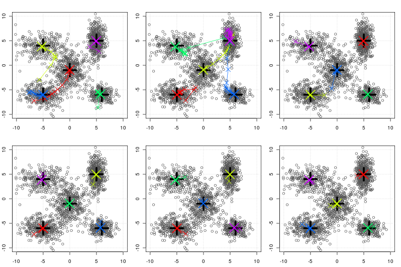
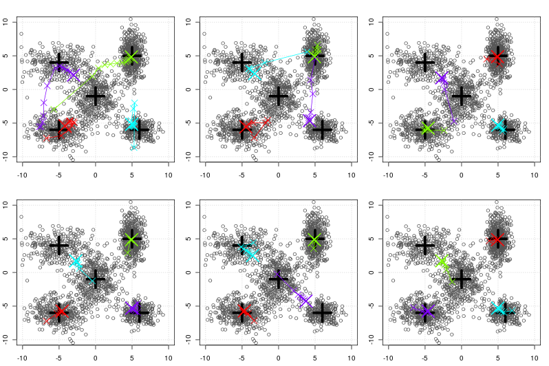
Below you see the artificial data produced by sampling from a 2 dimensional gaussian where the specified mean is denoted by the big horizontal/vertical black cross. The convergence of the (batch) k-means algorithm is shown by the colored traces for each iteration (batch). Each color corresponds to the convergence of a single centroid.
Obviously cleverly choosing initial centers can make a big difference. Nevertheless in a future posting we will see that in very high dimensions (as seen in the vector space model of IR) initialization does not seem to lead to fewer iterations or better local minima as it often does in low dimensions. This is another example of the so called Curse of dimensionality.

The k in k-means has been set to 5 centers. The upper three figures show k-means convergence when using three different random initialization on a data set of size 1771. Figures below show the convergence of k-means++. Obviously k-means++ starts with centers much closer to the true centers as in the case of random initialization.

The k in k-means has been set to 4 centers. The upper three figures show k-means convergence when using three different random initialization on a data set of size 1771. Figures below show the convergence of k-means++. Obviously k-means++ starts with centers much closer to the true centers as in the case of random initialization.