Hierarchical agglomerative clustering (HAC) is a family of different algorithms to perform grouping of data. HAC starts by merging the two data points with smallest distance into a new cluster and finishes with one big cluster describing the data.
The result of this merging process can be visualized by a so called dendrogram. In this post I sketch Ward's method or also called minimum variance method and show an example in the context of information retrieval.
Before we dive into hierarchical agglomerative clustering (HAC), let me state very shortly and informally, what we understand by clustering:
Given a set of data points in Euclidean space, a clustering algorithms tries to group similar points into clusters, so that each cluster is most homogeneous and at the same time the clusters should be well separated.
A hierarchical agglomerative clustering (HAC) algorithm starts with the single data points as trivial clusters by themselves and continues to merge cluster pairs which have minimum distance among all clusters until only a single cluster containing all data points is left (since the term agglomerative). The different algorithms can be distinguished by the specific distance function they apply to merge clusters.
Common to most HAC-algorithms is that they use a (dis)similarity matrix and have a run time complexity of \(\Omega(n^2)\) where \(n\) is the number of data points. The equation \(f = \Omega(g)\) means \((n) \geq g(n)\) for some \(n_0 \lt n\). For details see e.g. Wikipedia entry. As we see from the quadratic run time complexity HAC-algorithms are impractical on large problems. On the other hand we don't have to specify the number of clusters \(k\) in advance and get a lot more information about the structure of the data through the resulting "dendrogram" compared to common partitional clustering schemes like k-means clustering. For a general overview on clustering algorithms see e.g. Jain 99. For further information on hierarchical clustering see e.g. Fionn Murtagh 1985 (most of my further analysis is based on it).
Let \(P\), \(P^*\) be two partitions of the data points \(I={x_1,\ldots,x_n}\):
\[ \begin{eqnarray} P &:=& {p_1, \ldots, p_{k-1}, c_1, c_2}\nonumber\\ P^* &:=& {p_1, \ldots, p_{k-1}, c}\nonumber, \end{eqnarray} \]
where \(x_i\) are individual data points and \(p_i, c_i, c\) are sets (classes) of individual points. Then the variance of the data \(Var(I)\) (the squared deviation from the grand mean) is equal to the sum of between-class variance and the within-class variance:
\[ \begin{eqnarray} Var(I) &=& Var(P) + \left(\sum_{i=1}^{k-1} Var(p_i) + Var(c_1) + Var(c_2)\right)\nonumber\\ &=& Var(P^*) + \left(\sum_{i=1}^{k-1} Var(p_i) + Var(c)\right). \end{eqnarray} \]
It follows that the decrease in between-class variance when merging the clusters \(c_1\) and \(c_2\) into \(c\) is given by
\[ \begin{eqnarray}\label{bwvar} Var(P) - Var(P^*) &=& Var(c) - Var(c_1) - Var(c_2)\\ &=& \frac{|c_1||c_2|}{|c_1|+|c_2|}\|c_1-c_2\|^2, \end{eqnarray} \]
where \(c_i\) denotes the set of cluster members and also the respective centroids (means).
In minimum variance method, we seek to agglomerate two clusters \(c_1\) and \(c_2\), into cluster \(c\) such that the within-class variance of the partition thereby obtained is minimized. Equivalently the between-class variance of the obtained partition (see equation above) is maximized (see Murtagh p.70).
So the dissimilarity matrix at the start consists of all pairwise variances of the data points \(i,j\in {1,\ldots n}\):
\[ \begin{eqnarray}\label{sissim1} \frac{1}{2}\|i-j\|^2. \end{eqnarray} \]
To update the dissimilarity matrix after merging two objects \(i\) and \(j\), we can use the Lance-Williams dissimilarity update formula for Ward's method, which avoids costly calculations of the cluster means:
\[ \begin{eqnarray}\label{lance} d(i \cup j, k) &=& \frac{(|i|+|k|)d(i,k) + (|j|+|k|)d(j,k) - |k|d(i,j)}{|i|+|j|+|k|} \end{eqnarray} \]
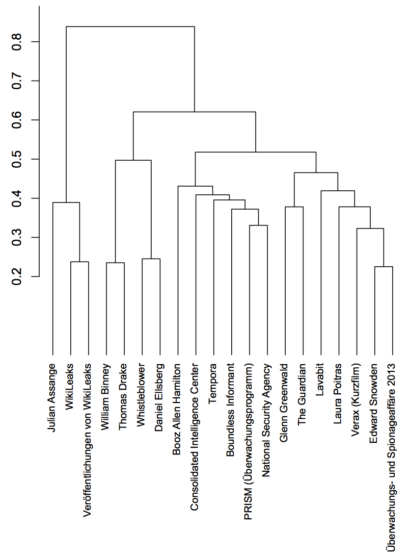
Here is an example from information retrieval (IR). Using the vector space model of IR, we can assign a vector to each document in a collection. Usually these vectors are normalized (to length 1), so that the inner product of two document vectors give us a measure of similarity. Using an own experimental search engine applying the vector space model on the german wikipedia collection of documents, we performed a query to retrieve the 20 most similar wikipedia articles for the article Edward Snowden. Then we build a dendrogram using the minimum variance criterium.
$ t(hc2$merge)
     [,1] [,2] [,3] [,4] [,5] [,6] [,7] [,8] [,9] [,10] [,11] [,12] [,13] [,14] [,15] [,16] [,17] [,18] [,19]
[1,]   -1  -10  -13   -4   -3   -5  -16  -14   -7   -11    -8   -19   -17    -6     8     2    14    16    10
[2,]   -2  -12  -20   -9    1  -15    6  -18    5     3     7    11     9    12    13     4    15    17    18
In R-project format singletons are negative and clusters of two more data points get a positive id. So first the singletons -1 "Edward Snowden" and -2 "Überwachungs- und Spionageaffäre 2013" are merged into cluster 1. In the 5-th merge the singleton -3 "Verax (Kurzfilm)" and the cluster 1 are merged into cluster 5.
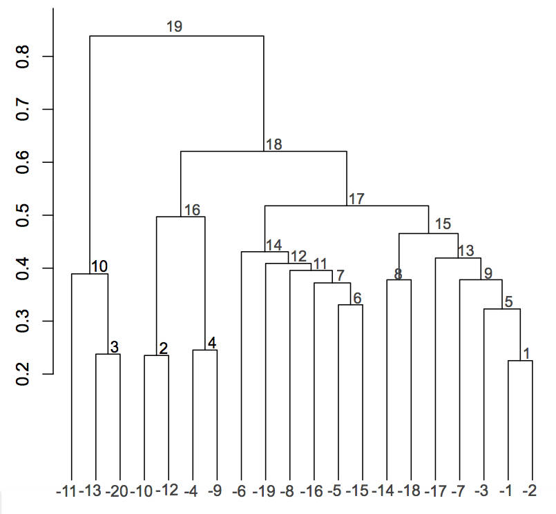
When looking at the above Dendrogram, it seems intuitive to choose e.g. the following 3 clusters as a compact representation of the clustering: 10, 16 and 17. Obviously we try to trade complexity of the clustering model for clustering error: The complexity of the cluster model is smallest when we have only a single cluster containing all data but the cluster error (variance) is biggest. When we have as much clusters as data points the clustering error is zero but the complexity of the cluster model is maximized. This leads to so called model based clustering, where the model complexity is choosen in a statistical consistent way using e.g. the Bayesian Information Criterium. Applying BIC to HAC may be the topic of a future post.